statduck
(ENCO)Efficient Neural Causal Discovery Without Acyclicity Constraints - review 본문
(ENCO)Efficient Neural Causal Discovery Without Acyclicity Constraints - review
statduck 2023. 7. 14. 22:50Contributions
Seperate paramemters and uses an objective unconstrained about acyclicity, which allows for easier optimization and low-variance gradient estimator having convergence guarantees
- Scaling to larger graphs and also can be leveraged to detect latent confounders
Background Knowledge
Causal Structure Learning : From sample of $\mathbb{P}$, discovering $G$ = causal structure learning or causal discovery. DAG 학습시키는게 목표이며 Data Set 종류로는 Observational Data, Interventional Data 존재.
Intervention Data 설명 https://www.inference.vc/causal-inference-2-illustrating-interventions-in-a-toy-example/
Joint distribtuion is not enough to predict behaviour under intervensions, however the causal diagram allows us to predict how the model will behave under intervention without carrying out the intervention.
Recent Work - continuous optimization score based causal discovery
- Search the space of possible graphs with gradient based mothods
- Adjacency matrix parameterized by independent probabilisites per edge
Method
- Score-base: Search thorugh all possible spaces
- Constrained-base: It constrains on functional class of SEM for identifiability result (like linear non-Gaussian acyclic model(LiNGAM), additive noise model(ANM) with conditional independence tests.
- Continuous-optimization (This paper adopts this method)
- Reinterpret Search as Discrete graph topology -> continuous problem
- Restrict the search space to acyclic graphs: Originally with lagrangian, regularizer which have cons like local optima problem and it can not scale over 100 variables
Restrition of acyclicity (Example) NOTEARS)


Problem :How to limit the search space to directed acyclic grpaph
To limit the search space,
- NOTEARS: $ h(W) = tr(e^{W\cdot W}) = 0$ (W is an adjacency matrix) (slow, param-sensitive)
- Regularization: penalize cyclic graphs (Hyperparameter sensitive and limited guarantees)
These two methods, however, have its own disadvantages.
Goal
- How can we reliably perform causal discovery with gradient-based methods on large scales?
- Find the DAG of causal graphical model(CGM) from observational and interventional samples
Central Idea : Learn distributions $p(X_1|...)$ from observational data, test generalization to interventional data
Parameterize graph with edge existence and orientation parameters
- Probability of an edge: $\sigma(\gamma_{ij}) \cdot \sigma(\theta_{ij}), \; with \; \theta_{ij}=-\theta_{ji}$
Benefits of two-variable parameterization:
- More control over gradient updates
- No constraint for acyclicity
And it leads to:
- Unbiased low-varaiance gradient estimators (-> able to scale larger)
- If intervene on all variables, global optima is guaranteed
Some Deifinitins CGM(Causal Graphical Models)
- DAG. G=(V,E)
- Random Variables $X = \{ X_1 ,..., X_N\}, \mathbb{P} = p(X)$
- Each node $i \in V = X_i $, edge $(i,j) \in E $ equals to causal relation $X_i \rightarrow X_j$
- $\mathbb{P}$ is faithful to a graph $G$ if the conditional independencies in $\mathbb{P}$ exactly equals to ones encoded in $G$ via d-separation https://blog.naver.com/sw4r/221004466858
- $\mathbb{P}$ is Markov to a graph $G$ if $p(X)$ can be factorized into $\Pi^N_{i=1} p_i (X_i | pa(X_i))$
- PGM(Probabilistic Graphical Model) based on DAG = BN(Bayesian Networks)
- CGM locally replaces $p_i(X_i|pa(X_i))$ by $\tilde{p}(X_i|pa(X_i))$. 이 때 $X_i$ = intervention target
- Intervention is perfect when $\tilde{p}(X_i|pa(X_i)) = \tilde{p}(X_i)$
Assumption
- The CGM is causally sufficient. (All common causes of variables are included and observable)
- We have N interventional datasets
- The interventions are sparse, perfect(indep of original parents), available for all observable variables
Learning Process

Distribution Fitting
At distribution fitting, it learns multiple conditional sets with drop-out from observational data. The bernollui parameter $p(X_j \rightarrow X_i)$ is updated at Graph fitting
Q: NN(Neural Network)에서 Conditional Density를 학습시키는 방법?
A. Leverage Normalizing flows for continuous variables, softmax output activiation for categorical variables.
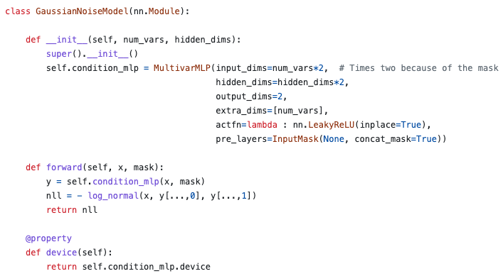
(Github에서 flow method 대신 simple way로 gaussiannoisemodel 제시: 분포 가정 후 파라미터 학습시키기: output_dims=2 loss function의 mean, log_var로 학습되도록)

Graph Fitting
- Sample a set of graphs(which doesn't have to be acyclic)
- Estimate log-likelihoods and average them for gradient estimators

Gradient Estimator
$$ \tilde{\mathcal{L}} = \mathbb{E}_{\hat{I} \sim p_I(I)} \mathbb{E}_{\tilde{p}_\hat{I}(X)} \mathbb{E}_{p_{\gamma,\theta} (C)} \Big[ \sum^N_{i=1} \mathcal{L}_C (X_i) \Big] + \lambda_{sparse} \sum^N_{i=1} \sum^N_{j=1} \sigma(\gamma_{ij}) \cdot \sigma(\theta_{ij}) $$
For Stochastic Gradient Descent method, we need to get the gradients for this form.
$$\dfrac{\partial}{\partial \gamma_{ij}} \tilde{\mathcal{L}} = \sigma(\gamma_{ij}) \cdot (1-\sigma(\gamma_{ij}))\cdot \sigma(\theta_{ij}) \cdot \mathbb{E}_{X,C_{-ij}}[ \mathcal{L}_{X_i \rightarrow X_j} (X_j) - \mathcal{L}_{X_i \nrightarrow X_j} (X_j) + \lambda_{sparse} ] $$
Evalulation
This paper evaluated 64,000 sampled adjacency matrix from $p_{\gamma,\theta}(C)$ in terms of log-likelihood estimates. These 64,000 samples are grouped into K samples(from 20 to 4,000 groups)
Low Variance For Edge Param($\gamma$)

Low Variance For Orientation Param ($\theta$)
In the learning process of $\theta$, regularizer doesn't need to be placed.
Because the $\theta$ parameter is only updated when intervention over index i,j so the other variables are not considered while learning at $ij$

Condition For global convergence
The main assumptions to converge globally are follows:


More intuitively speaking, Ancestors and descendants are not independent under interventions on the ancestor. Local optima only occur under this setting when there is a common confounder from parents, however this is not a usual case.
Score detecting latent confounders
Under latent confounder situation, the structure learning methods may predict false positive edges. (실제로는 관계가 없는데 있다고 착각할 수 있음)
Let $\gamma_{ij} = \gamma_{ij}^{(I)} + \gamma_{ij}^{(O)}$
$\gamma_{ij}^{(I)} $ is only updated under interventions on $X_i$

If this latent score is bigger than a threshold hyperparameter, then we can say there is a latent confounder between $X_i,X_j$.
Limitation
- Converengce guarantees require interventions on all variables
- Orientations are missing transitivity
Reference:
저자직강: https://www.youtube.com/watch?v=ro_5FqiS5qU
VAE 설명: https://process-mining.tistory.com/161
'Machine Learning' 카테고리의 다른 글
| Variational Inference (0) | 2023.08.17 |
|---|---|
| ML Study(1) - Kernel, Variational Inference, Tree methods (0) | 2023.08.07 |
| Bi-Tempered Logistic Loss (0) | 2023.04.11 |
| ChatGPT는 수능 수학을 풀 수 있을까?(오기편) (0) | 2023.02.12 |
| ChatGPT는 수능 수학을 풀 수 있을까? (0) | 2023.02.12 |


