statduck
Linear Method 본문
Problem Definition
| Cow | Milk(Y) | Age(X1) | Weight(X2) |
| #1 | 10 | 1 | 2 |
| #2 | 11 | 3 | 3 |
| #3 | 12 | 4 | 1 |
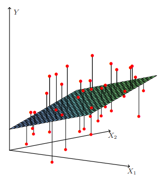
We want to find the model which well explains our target variable($y$) with $x$ variables. The model looks like this $$ Y_i =\beta_1X_{1i}+\beta_2X_{2i}+\epsilon_i $$
We can evaluate how precise our model it is with a fluctuation of our error. When we assume that our expected error is zero, the fluctuation represents the size of precision.
- Good for Intuition: $E[|\epsilon-E(\epsilon)|]=E[|\epsilon|]$
- Good for calculation: $\sqrt{E[\epsilon^2]}=\sigma_\epsilon$$
If we make a probabilistic assumption for error, we can easily find the fluctuation. For example, Error can be $-2, -1,0,1,2$ with the probability $\dfrac{1}{5}$. Then $E[|\epsilon|]=1$. However, in a real world problem, we couldn't make a probabilistic assumption for error. Even if we do, we just assume the normal with unknown variance. So to know the precision we need to estimate the sigma of error.
Coefficients(Beta)
Dive into $\hat{\beta}$
$\hat{\beta}^{LS}$ has $\mathbf{y}$ in its expression. When we assume the error follows probability distribution, $\mathbf{y}$ also becomes random variable that has uncertainty. Thus $\hat{\beta}^{LS}$ also follows a distribution related to the distribution of error.
Don't get confused! In a frequentist view, $\beta$ is constant. However the estimation value of beta $\hat{\beta}=f{(X_1,Y_1),...,(X_n,Y_n)}$ is a statistic so it has a distribution.
$$ \hat{\beta}=(\mathbf{X}^T\mathbf{X})^{-1}\mathbf{X}^T\mathbf{y} =(\mathbf{X}^T\mathbf{X})^{-1}\mathbf{X}^T(\mathbf{X}\beta+\epsilon) $$
$$ \hat{\beta}\sim N(\beta,(\mathbf{X}^T\mathbf{X})^{-1}\sigma^2) $$
$$ \hat{\sigma}^2=\dfrac{1}{N-p-1}\sum^N_{i=1}(y_i-\hat{y}i)^2 $$
$$ (N-p-1)\hat{\sigma}^2 \sim \sigma^2\chi^2{N-p-1} $$
Square of Normal becomes chi-square.
$$ z_j=\dfrac{\hat{\beta}_j}{\hat{sd}(\hat{\beta}_j)} =\dfrac{\hat{\beta}_j}{\hat{\sigma}\sqrt{v_j}} \sim t(df) \quad s.t. \; N-p-1 = df $$
$ \hat{Var}(\hat{\beta})=(X^TX)^{-1}\hat{\sigma}^2, \; \hat{Var}(\hat{\beta}j)=v_j\hat{\sigma}^2 \; v_j=j{th} \; diagonal \; element \; of \; (X^TX)^{-1} $
Now we know the distribution of test statistic $z_j$, so we can test whether the coefficient is zero and get the confidence interval. When we want to test whether subset of coefficients is zero, we can use the test statistic below.
$$
F=\dfrac{among \; group \; var}{within \; group \; var}=\dfrac{MSR}{MSE}=\dfrac{(RSS_0-RSS_1)/(p_1-p_0)}{RSS_1/(N-p_1-1)}
$$
$F$ has a distribution, so we can do zero value test for the coefficient. This testing gives hint for eliminating some input variables.
Gauss-Markov Theorem
This Theorem says Least Square estimates are good! There are three assumptions below.
- Input variables are fixed constant.
- $E(\varepsilon_i)=0$
- $Var(\varepsilon_i)=\sigma^2<\infty, \quad Cov(\varepsilon_i,\varepsilon_j)=0$
Under these assumptions, OLS is the best estimate by GM.(Refer to statkwon.github.io)
$$
E(\hat{\beta})=E(\tilde{\beta})=\beta $$
$$ Var(\tilde{\beta})- Var(\hat{\beta}) \;: positive \; semidefinite $$
Proof
https://en.wikipedia.org/wiki/Gauss%E2%80%93Markov_theorem
Always good?
$$ \begin{split} Err(x_0) ={}& E[(Y-\hat{f}(x_0))^2|X=x_0] \\
= \; & \sigma^2_\epsilon+[E\hat{f}(x_0)-f(x_0)]^2+E[\hat{f}(x_0)-E\hat{f}(x_0)]^2 \\
= \; & \sigma^2_\epsilon+Bias^2(\hat{f}(x_0))+Var(\hat{f}(x_0)) \\
= \; & Irreducible \; Error +Bias^2+Variance \end{split} $$
We can image the biased estimator away from old school OLS. By keeping more bias, we can lower much more variance. It means we more accurately predict future value.
Ridge, Lasso, and Elastic Net

Residual Sum of Squares
RSS - Error
Residual Sum of Squares is important. The more strict notation is error, not residual because Error is the random variable but residual is a constant after fitted.

$$ f(X)=\beta_0+X_1\beta_1+X_2\beta_2, \quad RSS(\beta)=(\mathbf{y}-\mathbf{X}\beta)^T(\mathbf{y}-\mathbf{X}\beta) $$
$$ \frac{\partial RSS}{\partial \beta}=-2\mathbf{X}^T(\mathbf{y}-\mathbf{X}\beta), \quad \frac{\partial^2 RSS}{\partial \beta \partial \beta^T}=-2\mathbf{X}^T\mathbf{X} $$
$$ (\mathbf{y}-\mathbf{X}\beta)^T(\mathbf{y}-\mathbf{X}\beta) = 0 \\ \mathbf{y}^T\mathbf{y} - \mathbf{y}^T\mathbf{X}\beta - \beta^T\mathbf{X}^T\mathbf{y}-\beta^T\mathbf{X}^T\mathbf{X}\beta=0 \\ -\mathbf{X}^T\mathbf{y}-\mathbf{X}^T\mathbf{y}-2\mathbf{X}^T\mathbf{X}\beta = 0 \\ -2\mathbf{X}^T(\mathbf{y}-\mathbf{X}\beta) = 0 $$
$$ \mathbf{X}^T(\mathbf{y}-\mathbf{X}\beta)=0, \quad \hat{\beta}=(\mathbf{X}^T\mathbf{X})^{-1}\mathbf{X}^T\mathbf{y} $$
$$ \hat{y}=\mathbf{X}\hat{\beta}=\mathbf{X}(\mathbf{X}^T\mathbf{X})^{-1}\mathbf{X}^T\mathbf{y}=\mathbf{H}\mathbf{y} $$
👀 Geometrical view

$Y$ is the projection onto the column space of $X$. This is because $\mathbf{H}$ is the projection matrix that has symmetric / idempotent properties. $\mathbf{H}$ is called as hat matrix (giving $y$ a hat)
| Q | A (Under the condition that $\hat{\beta} = \hat{\beta}^{LS}$ |
| What | $\mathbf{y}$ |
| Where | Column space of $\mathbf{X}$ |
| How | Projection |
$\varepsilon \perp x_i$, because $\epsilon=y-\hat{y}$. If we estimate $\beta$ in other methods with exclusion of $LSM$ method, the form $\hat{y}=\beta_0+X_1\beta_1+X_2\beta_2$ still remains. $\hat{y}$ is interpreted still as the vector on $\mathbf{col(X)}$. However, In this case $\hat{y}$ is not a projected vector so that the residual and variables are not orthogonal.
Regression
Variable Selection
This part is of selecting necessary independent variables. With several unnecessary variables, model has low predictive power and explanatory power. There are three ways to pick up the valuable variables:
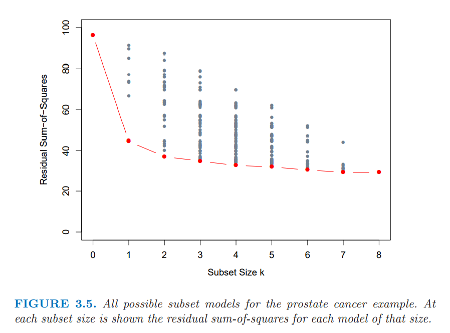
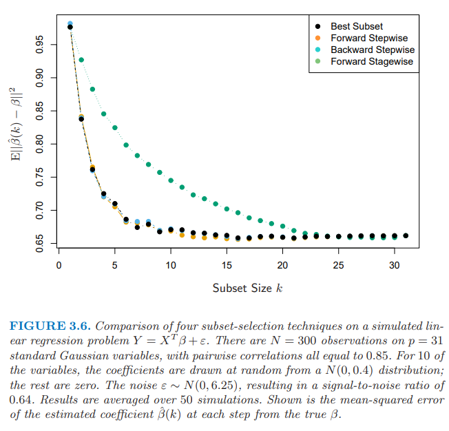
- Best Subset Selection
- Forward & Backward Stepwise Selection
- Forward Stagewise Regression
Best Subset Selection
$$
k \in {0,1,2,...,p}
$$
It is the method fitting every possible regression by subset size k. ( The optimal value in subset size 1 doesn't have to be optimal in size 2.)

Forward & Backward Stepwise Selection
Forward: Starting from zero model(Only intercept term exists), we put variables into our model one by one. This process could be done faster via QR decomposition.
Backward: Starting from Full model, we remove variables from our model one by one.

QR decomposition can lower our computational cost.
$$ X=QR, \quad X \in \mathbb{R}^{n\times p} ; Q\in \mathbb{R}^{n \times p} $$
$$ Q^T[X \quad y]=
\begin{bmatrix}
R \quad z \\ 0 \quad \rho \\ 0 \quad 0
\end{bmatrix} $$
$$ \hat{\beta}=(X^TX)^{-1}X^Ty=(R^TQ^TQR)^{-1}R^TQ^Ty=R^{-1}Q^Ty=R^{-1}z $$
$$ RSS(\hat{\beta})=||y-X\hat{\beta}||^2=z+\rho-y $$
$$ X_s=XS , \quad \beta_S=S^T\beta $$
$$ y=X_S\beta_S+\epsilon, \quad z=RS\beta_S+\xi $$
$$ \hat{\beta}=R_s^{-1}z_s, \quad RSS(\beta_S)=RSS(\hat{\beta})+\rho^2_S $$
Forward-Stagewise Regression
It is simliar with Forward-stepwise regression but has more constraints.
1) We pick the variable most correlated to the variable in our fitted model.
2) Let this variable be a target and the residual be an explanatory variable. Calculate the coefficient.
3) Adding this coefficient to the coefficient of our existing model.
Shrinkage
Variable Selection is a way to choose values in discrete way. The decision is only zero or one(removing or putting in). Because of this property, model variance would be increased. Shrinkage method is more free to variance because it choose variables in continuous way.
Lasso
$L_1$penalty is imposed.
$$
\hat{\beta}^{lasso}=argmin_\beta\sum^N_{i=1}(y_i-\beta_0-\sum^p_{j=1}x_{ij}\beta_j)^2, subject;to \sum^p_{j=1} |\beta_j| \leq t \
$$
Ridge
$$ \hat{\beta}^{ridge}=argmin_\beta\sum^N_{i=1}(y_i-\beta_0-\sum^p_{j=1}x_{ij}\beta_j)^2, subject;to \sum^p_{j=1} \beta_j^2 \leq t $$
$$ RSS(\lambda)=(y-X\beta)^T(y-X\beta)+\lambda \beta^T\beta $$
$$ \hat{\beta}^{ridge}=(X^TX+\lambda I)^{-1}X^Ty $$
$$ X=UDV^T $$
$$ X\hat{\beta}^{ls}=X(X^TX)^{-1}X^Ty = UU^Ty $$
$$ \begin{align*} X \hat{\beta}^{ridge} &= X(X^TX+\lambda I)^{-1}X^Ty \\ &= UD(D^2+\lambda I)^{-1}DU^Ty \\ &= \sum^p_{j=1} u_j \frac{d_j^2}{d_j^2+\lambda} u_j^Ty \end{align*} $$
Algorithm
By adding some processes, we can make a more elaborate model. Many algorithms make emphasize on the relationship between X variables and residual. $\hat{y}$ is on $col(X)$. With the view of linear combination, it is expressed as $\hat{y}=\hat{\beta_1}X_1+\hat{\beta_2}X_2+...+\hat{\beta_p}X_p$. The residuals is $\varepsilon = y-\hat{y}$. Our aim is to minimize $||\varepsilon||^2=\varepsilon \cdot \varepsilon$. What is the meaning of minimizing in terms of variable selection?
$$\begin{split} min(\varepsilon \cdot \varepsilon) & = min((y-\hat{y}) \cdot (y-\hat{y})) \\ & = min((y-(\hat{\beta_1}X_1+\hat{\beta_2}X_2))\cdot(y-(\hat{\beta_1}X_1+\hat{\beta_2}X_2))) \\ & =min((\hat{\beta_1}X_1 - y)\cdot \hat{\beta_2}X_2) \end{split}$$
$X_1$ is an existing variable and $X_2$ is a new variable.In this case, $y$ and $\hat{\beta_1}X_1$ are fixed and $\hat{\beta_2}X_2$ is an unfixed vector. Let's assume the norm of $\hat{\beta_2}X_2$ is fixed, and the direction is only changed. The important thing is the relationship between existing residual and $X_2$. Digging into the relationship between them is the key to decide whether the new variable would be put in or not. Many methods have been made from it.
LAR, PCR and PLS are representative examples. This algorithm is the method to make new features and the feature selection proceeds in such a way to minimize the error.
LAR(Least Angle Regression)
$$ y=\bar{y}+r $$
In this situation, we find $\beta_j$ of which $x_j$ has a high correlation with $r$
$$ y=\hat{\beta}_0+\hat{\beta}_1X_1+r, \; s.t. \; \hat{\beta}_1\in[0,\hat{\beta}_1^{LS}], \;s.t. \dfrac{x_j\cdot r}{||x_j||}<\dfrac{x_k\cdot r}{||x_k||}$$
Our fitted beta move from $0$ to $\hat{\beta}_1^{LS}$ until the correlation between another input variable and error becomes bigger. This approach makes beta come closer to the beta of least square, and the correlation between all input variables and error get reduced. This method can mine as many information as possible from our data. In the situation that $\hat{\beta}_j$ can't get close to $\hat{\beta}_j^{LS}$, $\hat{\beta}_j$ is fixed as $0$ like the Lasso regression.
Reference
Hastie, T., Tibshirani, R.,, Friedman, J. (2001). The Elements of Statistical Learning. New York, NY, USA: Springer New York Inc..
'Machine Learning' 카테고리의 다른 글
| Linear Classifier (1) (0) | 2022.05.27 |
|---|---|
| Orthogonalization (0) | 2022.05.27 |
| Statistical Decision Theory (0) | 2022.05.27 |
| Weighting procedure (0) | 2022.05.27 |
| Curse of dimensionality (0) | 2022.05.26 |


