Clustering & Nearest Neighbor

 

 Clustering is the method binding similar groups together. We can cluster customer type based on several variables about consumptions. In a mathematical expression, it means binding similar rows of a data matrix. For clustering, usually prototype methods are used. Prototype method assigns each observation to its closest prototype (centroid, medoid, etc.) "Closest" is defined by Euclidean distance in a feature space, after each feature has been standardized to have overall mean 0 and variance 1 in the training sample.

• It works well for capturing the distribution of each class.
• How many prototypes to use and where to put them are the main issues.

🕺 Goal: Partition the observations into clusters, so that the pairwise dissimilarities between points assigned to the same cluster becomes smaller than points in different clusters.

• Combinatorial Algorithm: Work without any probability model.
• Mixture modeling: Assume the data is an i.i.d sample from some population with probability function. The density function is expressed by a parameterized model.
• Mode seeking("bump hunters"): Directly estimate distinct modes of the probability density function. It takes a nonparametric perspective.

Dissimilarity

How can we define the similarity?

$$ D(x_i,x_{i'})=\sum^p_{j=1}d_j(x_{ij},x_{i'j})$$

Most of clustering methods take a dissimilarity matrix. By the attribute type, we can differently choose the shape of this function $d$.

• $d_j(x_{ij},x_{i'j})=(x_{ij}-x_{i'j})^2$
• Quantitative variables. $d(x_i,x_{i'})=l(|x_i-x_{i'}|)$
• Ordinal variables. $\frac{i-1/2}{M}, ;i=1,...,M$
• Categorical variables: $M \times M$ matrix with elements $L_{rr'}=1$ for all $r \neq r'$
• Minkowski distance: $d(x,y)={\sum^n_{i=1} (x_i-y_i)^p}^{1/p}$ (p=2: Euclidian)

How can we integrate all dissimilarity of attributes?

$$
D(x_i,x_{i'})=\sum^p_{j=1} w_j \cdot d_j(x_{ij},x_{i'j}), \; \;  \sum^p_{j=1} w_j=1
$$

 The influence of $X_j$on $D(x_i,x_{i'})$ depends upon its relative contribution to the average measure over all pairs of observation.

$$
\bar{D}=\dfrac{1}{N^2}\sum^N_{i=1}\sum^N_{i'=1}D(x_i,x_{i'})=\sum^p_{j=1}w_j\cdot \bar{d}_j, \; \bar{d}_j=\dfrac{1}{N^2} \sum^N_{i=1} \sum^N_{i'=1} d_j(x_{ij},x_{i'j})
$$

 Because $w_j \cdot \bar{d}_j$ is the relative influence of $j_{th}$variable, so setting $w_j \sim 1 / \bar{d}_j$ would give all attributes equal influence.

What is desired properties of dissimilarity function?

• Symmetry: $d(x,y)=d(y,x)$ Other wise you could claim "Alex looks like Bob, but Bob looks nothin Alex"
• Positive separability: $d(x,y)=0, ; if ;and ;only ;if ;x=y$ Otherwise there are objects that are different, but you cannot tell apart
• Triangular inequality: $d(x,y) \leq d(x,z)+d(z,y)$ Otherwise you could claim "Alex is very like Bob, and Alex is very like Carl, but Bob is very unlike Carl

Combinatory Algorithm

This algorithm assigns each observation to a cluster without regard to a probability model describing the data.

$$
W(C)-\dfrac{1}{2}\sum^K_{k=1}\sum_{C(i)=k}\sum_{C(i')=k} d(x_i,x_{i'})
$$

 

$$
T=\dfrac{1}{2} \sum^N_{i=1} \sum^N_{i'=1} d_{ii'}=\dfrac{1}{2}\sum^K_{k=1} \sum_{C(i)=k} \Big( \sum_{C(i')=k} d_{ii'}+\sum_{C(i')\neq k}d_{ii'} \Big) \\ T=W(C)+B(C), \; B(C)=\dfrac{1}{2} \sum^K_{k=1} \sum_{C(i)=k} \sum_{C(i')\neq k} d_{ii'}
$$

 

$W(C)$ stands for within-cluster and $B(C)$ for between-cluster. Our aim is to minimize $W(C)$ and maximize $B(C)$. Combinatory Algorithm needs to calculate all possible situations leading to an enormous inefficient computational speed.

$$
S(N,K)=\dfrac{1}{K!} \sum^K_{k=1}(-1)^{K-k} {K \choose k} k^N
$$

This value rapidly increases so we don't want to adopt this algorithm for large $N, K$

K-means Algorithm(Combinatory)

$$
d(x_i,x_{i'})=\sum^p_{j=1}(x_{ij}-x_{i'j})^2=||x_i-x_{i'}||^2 \\ W(C)=\dfrac{1}{2} \sum^K_{k=1} \sum_{C(i)=k} \sum_{C(i')=k} ||x_i-x_{i'}||^2=\sum^K_{k=1}N_k \sum_{C(i)=k} ||x_i-\bar{x}_k||^2
$$

• $\bar{x}k=(\bar{x}_{1k},...,\bar{x}_{pk})$ is the mean vector associated with $k_{th}$ cluster. Also it can be expressed as $c_j=(c_1,...,c_k)$
• $$N_k=\sum^N_{i=1}I(C(i)=k)$$, $$C(i)$$ is also expressed as $$\pi(i)$$

After we define our dissimilarity function, we can define the distort measure that we want to minimize for finding the closest centroids.

$$
J=\sum^N_{n=1}\sum^k_{j=1}\pi(i)||x_i-c_j||^2
$$

However, it is NP-hard problem so we need to adopt an iterative optimization way.

Algorithm[iterative descent algorithm]

🌻 Initialization Initialize k cluster centers, $\{c_1,\cdots,c_k\}$

🌻 Cluster assignment (Calculating the distance )

 $$\pi(i)=argmin_{j=1,\cdots,k}||x_i-c_j||^2$$

🌻 Center adjustment (Updating cluster center)

 $$c_j=\dfrac{1}{|\{i:\pi(i)=j\}|}\sum_{i:\pi(i)=j}x_i$$

Repeat assigning and adjusting until there is no change in $c_j$

K-means algorithm is usually used to find clusters from our unlabeled data. However, it also can be used to classify target variable from a labeled data.

1. Apply K-means algorithm to the training data in each class separately, using $R$ prototypes per class.
2. Assign a class label to each of the $K \times R$ prototypes. In this case, $K$ is the number of classes, and $R$ is the number of prototypes per class.
3. Classify a new feature $x$ to the class of the closest prototype.

 Learning Vector Quantization is used to correct the prototypes after we select prototypes. This method has the shortcoming that for each class, the other classes don't have a say in the positioning of the prototypes for that class.

Learning Vector Quantization(LVQ)

🌻 Initialization Initialize $R$ prototypes for each class: $m_1(k),\cdots,m_R(k)$

🌻 Sampling and adjusting Sample a training point $x_i$ randomly with replacement, and let $(j,k)$ be indicies the closest prototype $m_j(k)$ to $x_i$.

  🌻 If $$g_i=k, \; m_j(k) \leftarrow m_j(k)+\epsilon(x_i-m_j(k))$$

  🌻 if $$g_i \neq k, \; m_j(k) \leftarrow m_j(k)-\epsilon(x_i-m_j(k))$$

Repeat 2nd step, until the learning rate becomes 0.

 

 

Implementation From Scratch

import numpy as np
from PIL import Image
from random import *
import matplotlib.pyplot as plt

img_m = np.array(Image.open('data/myself.png'))
img_m = np.delete(img_m,obj=3,axis=2)

#train = 
#test = np.array([[1,1,5],[1,2,3],[2,3,10],[2,10,20],[2,10,40]])

def d(x,y,method=['l2']):
    if method=='l2': return (x-y)**2

class clustering():
    def __init__(self, data, data_dim):
        self.reshaped = data.reshape(-1,data_dim) # Flatten our data
        self.data_dim = data_dim

    def init_mean(self, num_cluster):
        seed(2020) # Random seed for reproducible result
        self.unique = np.unique(self.reshaped, axis=0)
        idx = sample(range(0,len(self.unique)), num_cluster) # Index sampling 
        self.ux = self.unique[idx] # Initializing value within data matrix
        ## Poor initialization
        # self.ux = np.array([np.random.uniform(0,1,self.data_dim) for num in range(num_cluster)])
        self.num_cluster = num_cluster

    def kmeans(self):
        # Second step: make a cluster variabe "r"
        self.u_pre = (self.ux)+0.1 # Just to make these difference in first step
        while np.sum(abs(self.u_pre - self.ux))>0.08:
            self.u_pre = (self.ux).copy()
            r = np.array([np.argmin(np.sum(d(x,self.ux,'l2'), axis=1)) for x in self.reshaped]) # r = array([k0,k2,k1,k1,...])
            # Third step: make a mean vector "ux"
            self.ux = [] # ux = [[k0 mean vec], [k1 mean vec], ...]
            for k in range(0,self.num_cluster):
                rk = (r==k).astype(int).reshape(-1,1) # rk = [[1],[0],[0],[0],...]] for np multiplication
                # Avoiding loop statement leads to reducing the time complexity
                u = (self.reshaped*rk).sum(axis=0)/(rk).sum(axis=0) # This solution is already given in our lecture.
                (self.ux).append(list(u)) # Binding u together.
            self.ux = np.array(self.ux)
        return(r, self.ux)

def kmeans_vis(data, num_cluster):
    km = clustering(data, 3)
    km.init_mean(num_cluster)
    r, uk = km.kmeans()
    reps = data.copy().reshape(-1,3)
    for i in range(num_cluster):
        reps[r==i] = uk[i]

    result = reps.reshape(data.shape[0], data.shape[1],3)
    plt.imshow(result, interpolation='nearest')
    plt.show()

 

Gaussian Mixtures

Setting :

$$
X|Z=e_k \sim N(\mu_k,\Sigma_k) \\ \where \; \mu_1,...,\mu_k\in \mathbb{R}^d, \; \Sigma_1,...,\Sigma_k\in \mathbb{R}^{d \times d}
$$

• $Z={e_1,e_2,\cdots,e_K}, ;e_1=[1 \;0 \; \cdots \; 0]^T$
• $p(X|Z=e_k)=N(X|\mu_k,\Sigma_k)=pdf \;of \;normal \; dist$
• $p(Z=e_k)=\pi_k =probability \;of \;selecting \; each \; cluster$
• $p(X)= \sum_z p(Z) \times p(X|Z)=\sum^K_{k=1} \pi_k \times N(X|\mu_k,\Sigma_k)$
• $p(X,Z)=p(Z) \times p(X|Z)=\pi_kN(X|\mu_k,\Sigma_k)$
• $p(Z=e_k|X)=\dfrac{p(Z) \times p(X|Z)}{p(X)}=\dfrac{\pi_k \times N(X|\mu_k,\Sigma_k)}{\sum^K_{j=1} \pi_j \times N(X|\mu_j,\Sigma_j)}=r(Z_{nk})$

def random_mat(n):
    x = np.random.normal(0, 0.1, size=(n, n))
    return x@np.transpose(x)

def params_init():
    params = {'pi': np.random.uniform(0,1),
    'mu': np.array([np.random.normal(0, 0.1, size=(5,)) for i in range(2)]), # k=2
    'sigma': np.array([random_mat(5)+np.identity(5) for i in range(2)])} #k=2
    return params

mu = params_init()['mu']; sigma = params_init()['sigma']
dist = [mvn(mean=mu[i], cov=sigma[i]) for i in range(2)]

# PCA
scaler = StandardScaler()
scaler.fit(df)
X_scaled = scaler.transform(df)
cov_matrix = np.cov(X_scaled.T)
eigvals, eigvecs = np.linalg.eig(cov_matrix)
eigvec_mat = (eigvecs.T[:][:5]).T
X_pca = (X_scaled @ eigvec_mat / eigvals[:5]).astype(float)

obj = []

def e_step(x, params, i):
  pi = params['pi']; mu = params['mu']; sigma = params['sigma']
  dist = [mvn(mean=mu[i], cov=sigma[i]) for i in range(2)]
  r_vec = [[( pi * dist[k].pdf(x[i]) ) / ((pi * dist[0].pdf(x[i]))+ ((1-pi)*dist[1].pdf(x[i]))) for i in range(x.shape[0])] for k in [0,1]]
  clst = [ int(r_vec[0][i] < r_vec[1][i]) for i in range(x.shape[0])]
  # Originally, calculating log-likelihood is the step after m_step
  # But for computational convenience, I put it in this e_step.
  log_likelihood = sum([np.log( pi * dist[0].pdf(x[i]) + (1-pi)*dist[1].pdf(x[i])) for i in range(x.shape[0])])
  obj.append(log_likelihood)
  return np.array(r_vec), clst

def m_step(x, params, r_vec):
  N = r_vec.sum(axis=1)
  elem = np.dot(r_vec,x)
  mu = np.array([elem[0]/N[0] , elem[1]/N[1]])
  pi = (N/N.sum())[0]
  sigma = [(1/N[k]) * np.array([ r_vec[k][i] * (np.outer(X_pca[i] - params['mu'][k],X_pca[i] - params['mu'][k]))
  for i in range(X_pca.shape[0])]).sum(axis=0)
  for k in range(2)]
  params = {'pi':pi, 'mu':mu, 'sigma':np.array(sigma)}
  return params

 i = 0
 params = params_init()
 while i<50:
     i += 1
     r_vec, clst = e_step(X_pca, params,i)
     params = m_step(X_pca, params, r_vec)

fig, ax = plt.subplots()
ax.plot(range(i), obj, marker='.', color='r')
ax.grid(True)
ax.set_xlabel('# of iteration')
ax.set_ylabel('log likelihood')
ax.set_title('log likelihood')
plt.show()

 

 

Algorithm[EM Algorithm]

🌻 Initialization Initialize the means $\mu_k$, covariance $\Sigma_k$ and mixing coefficients $\pi_k$.

🌻 E step Evaluate $r(z_{nk})=\dfrac{\pi_k N(x_n|\mu_k,\Sigma_k)}{\sum^K_{j=1} \pi_j N(x_n|\mu_j, \Sigma_j)}$

🌻 M step Re-estimate the parameters using $r(z_{nk})$

$$\mu_k^{new}=\dfrac{1}{N_k}\sum^N_{i=1}\gamma(z_{nk})x_n$$

$$\Sigma_k^{new}=\dfrac{1}{N_k}\sum^N_{i=1}\gamma(z_{nk})(x_n-\mu_k^{new})(x_n-\mu_k^{new})^T$$

$$\pi_k^{new}=\dfrac{N_k}{N}, ;; s.t ; N_k=\sum^N_{n=1}\gamma(z_{nk})$$

🌻 Evaluation Evaluate the log likelihood

$$ln p(X|\mu,\Sigma,\pi)=\sum^N_{n=1}ln{\sum^K_{k=1}\pi_k N(x_n|\mu_k,\Sigma_k)}$$

  Check for convergence of either the parameters or the log likelihood. If the convergence criterion is not satisfied return to E step. $r(z_{nk})$ means responsibility.

 

K-medoids

K-means cluster has following two flaws.

• [Lack of Robustness] Euclidean distance places the highest influence on the largest distance leading to lack of robustness.
• [Only For Numerical Variables] It is impossible to compute arithmetic mean for a categorical feature.

To handle with these two problems, K-medoids can be used. This way

$$
J=\sum^n_{i=1}\sum^p_{j=1}r_{ij}D(x_i,\mu_j)
$$

• $r_{ij}=1$ if $x_i$ belongs to $j$ cluster. (otherwise the value becomes $0$)
• $D(x_i,\mu_j)$, $\mu_j$ is the mean vector in $j$ cluster.

Algorithm

🌻 Initialization a set of cluster centers: ${m_1,...,m_K}$, and assignment $C$

🌻 Cluster Assignment $ i^*k=argmin{i:C(i)=k} \sum_{C(i')=k}D(x_i,x_{i'})$

 

🌻 Center Update

 

$$C(i)=argmin_{1 \leq k \le K}D(x_i,m_k)$$

Iterate Assigning/Updating until the assignments do not change.

In this algorithm, we don't need to compute the cluster center so we can use categorical variables also. We just need to keep track of the indices $i_k^$

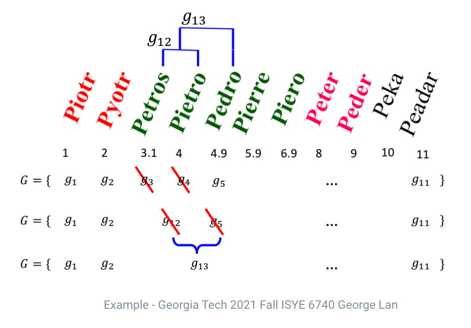
Hierarchical Clustering

Hierarchy in cluster mean that at the lowest level each cluster contains only one single point but at the highest level there is only one cluster containing all of the data. Hierarchical clustering composes of two steps:

• Agglomerative(bottom-up): It starts at the bottom and at each level it recursively merge a selected pair of clusters into a single cluster.
• Divisive(top-down): It starts at the top and at each level it recursively split one of the existing clusters at that level into two new clusters.

For visualization tool, dendrogram is usually used. I only handle bottom-up model in this chapter. The algorithms is as follows.

Algorithm

🌻 Assigning: Assign each data point to its own cluster, $g_1 = {x_1},...,g_m={x_m}$

let $G={g_1,...,g_m}$

🌻 Do:

• Find two clusters to merge: $i,j=argmin_{1\leq i, j \leq |G|} D(g_i,g_j)$
• Merge the two clusters to a new cluster: $g \leftarrow g_i \cup g_j$
• Remove the merged clusters: $G \leftarrow G(g_i), \;G \leftarrow G(g_j)$
• Add the new clusters: $G \leftarrow G \cup {g}$

🌻 While $|G|>1$

 

 

• Single Linkage: $d_{SL}(G,H)=\min_{i\in G, i' \in H} d_{ii'}$
• Complete Linkage: $d_{CL}(G,H)=min_{i\in G, i' \in H} d_{ii'}$
• Group Average: $d_{GA}(G,H)=\dfrac{1}{N_G N_H}\sum_{i \in G} \sum_{i' \in H} d_{ii'}$, $N_G, N_H$ are the number of observations in each group. (This method is similar with K-means clustering)

This type of cluster can be done with single linkage, because it uses a minimum distance.

Nearest Neighbor

 Nearest Neighbor is the way to classify or predict a target data of a new point X by leveraging data near by this new point. This method regulates the weight of each data by distance.

 Our goal is to determine the number of class $k$ to be large enough to minimize an error, and to be small to give an accurate estimation. I'm gonna show that the class of $k-NN$ rules, the single nearest neighbor rule is admissible by showing that there exists no $k-NN$ rule, $k\neq 1$, which has lower probability of error against all distributions for the $n$ sample problem.

 Let me consider the situation that the prior probabilities $\eta_1 = \eta_2 = \dfrac{1}{2}$, and data points in each class are well separated. Also, the number of category is only two, so each data point is assigned into category 1 or 2. This problem can also be thought as the binomial situation, which each trial has just success or fail. Under this condition, I'll show that $1-NN$ rule is strictly better than the $k-NN$ rule in the case where the densities are clearly separated.

• The probability that $j$ individuals come from category 1: $(\dfrac{1}{2})^n {n \choose j}$
• $P_\epsilon(1;n)$ is the error that all points lie in category 2: $(\dfrac{1}{2})^n$
• $P_\epsilon(k;n)=(\dfrac{1}{2})^n\sum^{k_0}_{j=0} {n \choose j}, ;; s.t. ; k=2k_0+1$. It means the probability that $k_0$ or fewer points lie in category 1

When the new data point $x$ is actually in a category 1, only if the $k_0$ nearest points or fewer points are in a category 2, this point $x$ is assigned into a category 1. This is the situation of choosing $k_0$ points as 2 and other points as 1.

 

Practical Issues

How can we decide the number of clusters?

Gap Statistic

We can leverage the within cluster dissimilarity $W_k$

• $K\in {1,2,...,K_{max}}, \; W={W_1,W_2,...,W_{K_{max}}}$
• $K^{*}=argmin_K{K|G(K) \geq G(K+1)-s'_{K+1}}$

Reference [Gap statistic]

Silhouette value

We can also use a Silhouette value $S_i = \dfrac{b_i-a_i}{max(a_i,b_i)}$ . $a_i$is the average distance from the $i$th data point to the other points in the same cluster, and $b_i$ is the minimum average distance from the $i$th point to points in a different cluster. When our groups are well clustered, $b_i-a_i$ has to become big.