Latent Factor Model

    The basic assumption is that significant portion of the rows and columns of data matrix are highly correlated. Highly correlated data can be well explained by a low number of columns, so low-rank matrix is useful for the matrix estimation. It reduces the dimensionality by rotating the axis system, so that pairwise correlations between dimensions are removed.

 

Low Rank Approach 

✏️ $R$ has a rank $k <\!\!<min\{m,n\}$

$$ R=UV^T $$

- $U$ is an $m \times k$ matrix, and $V$ is a $n \times k$ matrix.
- Each column of $U$ is viewed as one of the $k$ basis vectors.
- $j_{th}$row of $V$ contains the corresponding coefficients to combine basis vectors.

✏️$R$ has a rank larger than $k$
$$
R \approx UV^T
$$

    The residual matrix is $(R-UV^T)$ and the error is $||R-UV^T||^2$. In this situation $|| \cdot ||$ is the Frobenius norm(It calculates the sum of the squares for every entries).

 

    In this case the genre becomes the latent vector(concept). In this chapter, we want to find the elements in $U$ and $V$ matrix by solving an optimization problem.

 

 

Geometric Intuition

    Let's assume the ratings of these three movies are highly positively correlated. In this case, just one latent factor is enough to explain the trend of a data. When we know just one rating score, we can also know the other ratings of other movies by finding the intersection point between a plane and a vector.
    The thing is that we focus on finding a set of relevant latent vector. The averaged squared distance of the data points from the hyperplane defined by these latent vectors must be as small as possible.

Basic Matrix Factorization

$$ R\approx UV^T, \;\; r_{ij}\approx \vec{u_i}\cdot \vec{v_j} $$
- The $i$th row $\bar{u_i}$ of $U$ is a user factor, which has the affinity with user $i$ towards $k$ concepts.
- Each row $\bar{v_i}$ of $V$ is an item factor, which has the affinity with $i$th item towards $k$ concepts.

$$ r_{ij}\approx \sum^k_{s=1}u_{is} \cdot v_{js} $$
    In the example above, $r_{ij}$ has the meaning as follows. The sum of (Affinity of user $i$ to _history_)$\times$(Affinity of item $j$ to _history_) and (Affinity of user $i$ to _romance_) $\times$(Affinity of item $j$to _romance_) When $U,V$have negative values, it becomes hard to interpret the meaning of a latent vector. To make the model interpretable, NMF(Non-negative Matrix Factorization) is introduced in the following post.

 

Unconstrained Matrix Factorization

    Even SVD(Singular Vector Decomposition) has a constraint that each vector is orthogonal. In this chapter, we handle with an unconstraint problem.

$$ Minimize \;J=\dfrac{1}{2}||R-UV^T||^2 $$

$$ Minimize \; J=\dfrac{1}{2}\sum_{(i,j)\in S}e^2_{ij}=\dfrac{1}{2}\sum_{(i,j)\in S}(r_{ij}-\sum^k_{s=1}u_{is}\cdot v_{js})^2 $$

    Because of missing entries, only a subset of entries are known. $\sum^k_{s=1}u_{is}\cdot v_{js}$ means the similarity between user $i$ and item $j$ for every latent variables. To clarify the objective function, we need to consider only a set known as follows.
$$
S=\{(i,j):r_{ij}\; is \;observed\}
$$

 

- $q$ denotes the index of latent variables.
- $\nabla J=[\dfrac{\partial J}{\partial u_{iq}} \; | \; \dfrac{\partial J}{\partial v_{jq}} ], \; \; VAR=[U \; | \; V]=VAR-\alpha\cdot \nabla J$
- As a matrix form, $U\Leftarrow U+\alpha EV; \; V\Leftarrow V+\alpha E^TU$

 

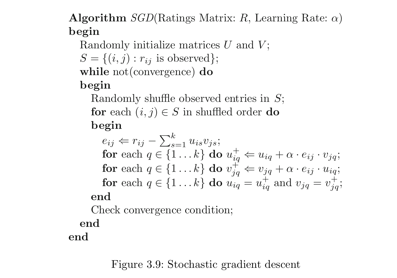
    Different from the update method above, SGD can update entries in matrices by only using a part of a set $S$.

- As a vector form, $\vec{u_i} \Leftarrow \vec{u_i}+\alpha e_{ij} \vec{v_j}, \; \vec{v_j}\Leftarrow \vec{v_j}+\alpha e_{ij}\vec{u_i}$
- For one update, a single observed entry $(i,j)$ is needed.

    In practice, SGD can achieve faster convergence than GD, but GD can have more smoother convergence. $\alpha$ is usually determined as 0.005. To avoid local optimum problem, it also adopts bold driver algorithm(Selection for $\alpha$ for each iteration.) Initialization is also issue, and one can handle this issue with SVD-based heuristic dealt with later section. The basic idea of regularization is to discourage very large entries in $U$and $V$by adding a regularization term, $\dfrac{\lambda}{2}(||U||^2+||V||^2)$ into the optimization problem. In this case the regularization term is $L_2$

 

✏️Gradient Descent

$$U \Leftarrow U(1-\alpha \cdot \lambda)+\alpha EV, \; V \Leftarrow V(1-\alpha \cdot \lambda)+\alpha E^TU$$

    In which unobserved entries of $E$ are set to $0$. $(1-\alpha \cdot \lambda)$plays a role in shirking the parameters in each step.

 

✏️Stochastic gradient descent - vectorized local updates

$$\vec{u_i}\Leftarrow \vec{u_i}+\alpha(e_{ij}\vec{v_j}-\lambda \vec{u_i}),\; \vec{v_j} \Leftarrow \vec{v_j}+\alpha(e_{ij}\vec{u_i}-\lambda \vec{v_j})$$

    We can also update our parameter using a vector form in stochastic gradient descent.

✏️Stochastic gradient descent - vectorized global updates

$$ \vec{u_i}\Leftarrow \vec{u_i}+\alpha(e_{ij}\vec{v_j}-\lambda\vec{u_i}/n^{user}_i), \; \vec{v_j}\Leftarrow \vec{v_j}+\alpha(e_{ij}\vec{u_i}-\lambda\vec{v_j}/n^{item}_j) $$

    The regularization term is divided by the corresponding observed entries. The book said the local update use $u_{iq}$ and $v_{jq}$ several times, while the global update use these variable just once. It leads to difference between two methods.(Trade-offs between quality and efficiency) It's also possible to train the latent components incrementally. The approach repeatedly cycles through all the observed entries in $S$ while performing theses updates for $q=1$ until convergence is reached.

$$ R\approx UV^T=\sum^k_{q=1}\vec{U_q}\vec{V_q}^T $$



- The result means that overall rank-k factorization can be expressed as the sum of k rank-1 factorization.
- $\vec{U_q}\vec{V_q}^T$ is an outer product of $U_q$ and $V_q$.
- The main difference between this approach and the approach above is that it cycles through in $q$ in the outer loop.
- This approach leads to faster and more stable convergence.
- The earlier latent components become the dominant ones, like they do in SVD.(Even if this approach doesn't ensure the orthogonality between vectors, but it can make these vectors orthogonal using projected gradient descent.)



The stochastic gradient method is sensitive both to the initialization and the way in which the step sizes are chosen. To compensate for these shortcomings, ALS can be applied.

Algorithm for ALS

- Keeping $U$ fixed. In the optimization problem, $\sum_{i:(i,j)\in S}(r_{ij}-\sum^k_{s=1}u_{is}v_{js})^2$, $u_{i1},...,u_{ik}$are treated as constant, whereas $v_{j1},...,v_{jk}$ are treated as variables. It becomes a least-square regression problem in $v$.
- Keeping $V$ fixed. $v_{j1},...,v_{jk}$ are treated as constant, where as $u_{i1},...,u_{ik}$ are treated as variables.

    These two steps are iterated to convergence. The least squares problem for each user is independent, so that this step can be parallelized easily.


 A weighted version ALS can be well-suited to implicit feedback settings where the matrix is assumed to be fully specified with many zero values. However, ALS is not quite as efficient as stochastic gradient descent in large-scale settings with explicit ratings. Other methods such as coordinate descent can address this problem.

 

 

Updates for coordinate descent
$$u_{iq} \Leftarrow \dfrac{\sum_{j:(i,j)\in S}(e_{ij}+u_{iq}v_{jq})v_{jq}}{\lambda+\sum_{j:(i,j)\in S}v^2_{jq}}$$
$$v_{jq} \Leftarrow \dfrac{\sum_{i:(i,j)\in S}(e_{ij}+u_{iq}v_{jq})u_{iq}}{\lambda+\sum_{:(i,j)\in S}u^2_{iq}}$$

 

Singular Value Decomposition

 

Consider the rating matrix is fully specified. One can approximate R by using truncated SVD of rank $k <\!\!< min\{m,n\}$

$$
R\approx Q_k\Sigma_kP_k^T
$$

- $Q_k$ contains the $k$ largest eigenvectors of $RR^T$
- $P_k$ contains the $k$ largest eigenvectors of $R^TR$. $P_k$ represents the reduced row space, $k$ eigenvectors imply the directions of item-item correlations among ratings.
- $Q_k\Sigma_k$ contains the transformed and reduced $m\times k$ representation of the original rating matrix
- $U=Q_k\Sigma_k, \;\; V=P_k$

    When $R$ is incompletely specified, one can impute missing entries by using row-wise average.

How to execute
1. Let the centered matrix $R_c$, let missing entries of $R_c$ be $0$.
2. Decompose $R_c$ into $Q_k\Sigma_kP_k^T$
3. $U=Q_k\Sigma_k,\;\;V=P_k$
4. $\hat{r}_{ij}=\bar{u}_i\cdot\bar{v}_j+\mu_i$