statduck
Linear Classfier (2) 본문
Calculation

$$ \delta_k(x) =-\dfrac{1}{2}log|\hat{\Sigma}_k|-\dfrac{1}{2}(x-\mu_k)^T\hat{\Sigma}_k^{-1}(x-\mu_k)+log\pi_k $$
$\hat{\Sigma}_k=U_kD_kU_k^T$can make this calculation more faster.
$$
✔️ (x-\hat{\mu}k)^T\hat{\Sigma}^{-1}_k(x-\hat{\mu}_k)=[U_k^T(x-\hat{\mu}_k)]^TD_k^{-1}[U_k^T(x-\hat{\mu}_k)] \
✔️ log|\hat{\Sigma}_k|=\Sigma_llogd{kl}$$
In normal dsitrubiton, the quadratic form means mahalanobis distance. This is the distance that(https://darkpgmr.tistory.com/41) how much each data is away from the mean over the standard deviation.
$$
X^=D^{-1/2}U^TX \\
Cov(X^)=Cov(D^{-1/2}U^TX)=I
$$
Using this expression, we can interpret it as assigning $X^*$ to the loc $\mu^*$. The mahalanobis distance can be changed into euclidiean distance. In a transformed space, each point is assigned into a closest median point. It controls the effect of prior probability($\pi_k$). The transformed space $X^*$ is equivalent to Whitening transformation that changes the variance of X into $\mathbf{I}$.
$$ Y=WX, \; W^TW=\Sigma^{-1} \; D^{-1/2}U^T=W $$

High Dimensional Data
- $p$: The dimension of input matrix
- $K$: The number of centroid.
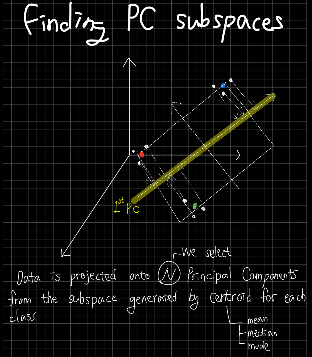
LDA(QDA) reduces the $p$ dimensional space into $K$ centroids, thereby reducing the dimensionality of the problem to $K-1$. Let $H_{K-1}$ be the subspace spanned by these centroids. Since the centroids are already in this subsapce, the distance between $H_{K-1}$ and $X^*$can be neglected, as it has the same impact on all the centorids.
To find the optimal subspace, we can project the transformed $X^*$onto $H_{K-1}$, and compare distance between the projected points. If the variance of these projected centroids is large, then it is an optimal situation. Finding the optimal subspace is equivalent to finding PC space of centroids.
- Class centroids $\mathbf{M} \;(K \times p)$ , Common covariance matrix $\mathbf{W}=\hat{\Sigma}=\Sigma^K_{k=1}\Sigma_{g_i=k}(x_i-\hat{\mu}_k)(x_i-\hat{\mu}_k)^T/(N-K)$
- $\mathbf{M}^*=\mathbf{MW}^{-1/2}$ using the eigen-decomposition of $\mathbf{W}$
- $\mathbf{B}^*=Cov(\mathbf{M}^*)=\mathbf{V^*D}_B\mathbf{V}^{*T}$, Columns of $\mathbf{V}^{*T}$are $v_l^*$
- $Z_l=v_l^TX ; with ; v_l=\mathbf{W}^{-1/2}v_l^*$
- $\mathbf{W}$: Within-variance matrix, $\mathbf{B}$: Between-variance matrix
Find the linear combination $Z=a^TX$such that the between-class variance is maximized relative to the within-class variance. We can reformulate the problem as follows:
$$
max_a\dfrac{a^TBa}{a^TWa} \\
max_aa^TBa \quad subject \;\; to \;\; a^TWa=1
$$
The solution $a$ becomes the biggest eigenvector of $W^{-1}B$. We can represent our data in a reduced form using the axis of $Z_l=v_l^TX=a_l^TX$. $Z_l$ is called as a canonical variate and this becomes a new axis.
RDA
✏️ Definition
RDA(Regularized Discriminant Analysis) is the combinational model between LDA and QDA.
$$
\hat{\Sigma}_k(\alpha)=\alpha\hat{\Sigma}_k+(1-\alpha)\hat{\Sigma}, \quad \alpha \in[0,1]
$$
Expressing form with a vector internal division is a most common way in combinational model. $\hat{\Sigma}$ is a pooled covariance matrix from LDA. If we replace $\hat{\Sigma}$ as $\hat{\Sigma}(\gamma)$, this also can be changed into $\hat{\Sigma}(\alpha,\gamma)$. For generalization, parameter is just added.
$$
\hat{\Sigma}(\gamma)=\gamma\hat{\Sigma}+(1-\gamma)\hat{\sigma}^2I, \quad \gamma \in[0,1]
$$
$\hat{\sigma}^2I$ also can be changed into $diag(\hat{\Sigma}), \hat{\Sigma}/p,...$

Support Vector Machine
Classification Problem

$$ y(x)=w^Tx+b $$
This line is a decision boundary. We define a margin as the perpendicular distance between the line and the closet data point. We just want to find the line maximizing the margin.
$$
\max_{w,b} \dfrac{2c}{||w||}, \; s.t. \;y_i(w^Tx_i+b)\geq c, \forall i
$$
This problem easily changes into the problem because c just changes the scale of w and b.
$$
\max_{w,b} \dfrac{1}{||w||}, \; s.t.\; y_i(w^Tx_i+b) \geq1,\forall i
$$
It is equal to a constrained convex quadratic problem.
$$
\min_{w,b} ||w||^2, \; s.t. \; y_i(w^Tx_i+b) \geq 1, \forall i \\ L(w,b,\alpha)=||w||^2+\sum_i\alpha_i(y_i(w^Tx_i+b)-1)
$$
This primal problem can be changed into a dual problem.
$$
\min_{w,b} \dfrac{1}{2}w^Tw, \; s.t. \; 1-y_i(w^Tx_i+b) \leq0, \forall i \ L(w,b,\alpha)=\dfrac{1}{2}w^Tw+\sum_i\alpha_i(1-y_i(w^Tx_i+b))
$$
By Taking derivative and set to zero,
$$
\dfrac{\partial L}{\partial w}=w-\sum_i\alpha_iy_ix_i=0 \\ \dfrac{\partial L}{\partial b}=\sum_i \alpha_iy_i=0
$$
Using these equations, the problem becomes more easy
$$
L(w,b,\alpha)=\sum_i \alpha_i-\dfrac{1}{2}\sum_{i,j}\alpha_i\alpha_jy_iy_j(x_i^Tx_j), \\ s.t. \; \alpha_i \geq 0, \; \sum_i \alpha_i y_i =0
$$
This is a constrained quadratic programming.
KKT condition(1)
In the KKT condition, there is the condition $\alpha_i g_i(w)=0$. $$ \alpha_i(1-y_i(w^Tx_i+b))=0$$
alpha can be zero, or the other can be zero. When alpha is nonzero, the train points supposed to be on a decision line are called support vectors.
KKT condition(2)
$\dfrac{\partial L}{\partial w}=0$, so $w=\sum_i \alpha_iy_ix_i$. For a new test point z, we need to compute this
$$
w^Tz+b=\sum_{i \in support \; vectors} \alpha_iy_i(x_iz)+b
$$
$b$ can be derived from $1-y_i(w^Tx_i+b)=0, \; with \; \alpha_i>0$
Problem 1
Data could be not linearly separable. In this case we use this.
$$ (w^Tx+b)y \geq 1-\xi $$
$$ \min_{w,b,\xi} ||w||^2+C\sum_i \xi_i, \; s.t.\; y_i(w^Tx_i+b)\geq1-\xi_i, \; \xi_i \geq 0, \forall i $$
$$ \min_{w,b} \dfrac{1}{2}w^Tw, \; s.t. \; 1-y_i(w^Tx_i+b)-\xi_i \leq0, \; \xi_i \geq 0, \forall i $$
$$ L(w,b,\alpha,\beta)=\dfrac{1}{2}w^Tw+\sum_i C\xi_i+\alpha_i(1-y_i(w^Tx_i+b)-\xi_i)-\beta_i\xi_i $$
$$ L(w,b,\alpha,\beta)=\sum_i\alpha_i-\dfrac{1}{2}\sum_{i,j}\alpha_i\alpha_jy_iy_j(x_i^Tx_j) $$
$$ \max_\alpha \sum_i \alpha_i - \dfrac{1}{2} \sum_{i,j} \alpha_i \alpha_j y_i y_j (x_i^Tx_j) $$
$$ s.t. C-\alpha_i-\beta_i=0, ; \alpha_i \geq 0, ; \beta_i \geq 0, i=1,...,m, \sum_i \alpha_iy_i=0 $$
It is also a constrained quadratic programming.
Soft margin SVM with primal form
$$
\min_{w,b,\xi} ||w||^2+C \sum_i \xi_i \ s.t. ; y_i(w^Tx_i+b) \geq 1-\xi_i, \xi_i \geq 0, \forall i
$$
$$\min_{w,b} ||w||^2+C\sum_i max{0,1-y_i(w^Tx_i+b)}$$
It is an unconstrained strong convex problem, but not necessarily differentiable. Because it doesn't be differentiable over domain, we use subgradient method instead of original gradient method. Anyway, this gradient method is used to find the optimal w. $b$ is solved by this equation:
$$1-y_i(w^Tx_i+b)=0$$
$$J(w,b) = ||w||^2+C\sum max{0,1-y_i(w^Tx_i+b)}$$
$$
\nabla^{sub}_w J(w,b)=w-C\sum_i \begin{cases} 0, & 1-y_i(w^Tx_i+b) \leq 0 \\ y_ix_i, & 1-y_i(w^Tx_i+b)>0 \end{cases}
$$
$$
\nabla^{sub}_b J(w,b)=-C\sum_i\begin{cases} 0, & 1-y_i(w^Tx_i+b) \leq 0 \\ y_i, & 1-y_i(w^Tx_i+b)>0 \end{cases}
$$
$w^{new}=w^{old}-\eta \nabla^{sub}{w}J(w,b), ; ; b^{new}=b^{old}-\eta \nabla^{sub}{b}J(w,b)$
Subgradient method
$$ f(x)=|x| $$
g is a subgradient of $f: X\rightarrow R, \; x\in X$, for any $y \in X, f(y) \geq f(x) + \langle g,y-x \rangle $
Regression Problem
$$ f(x)=x^T\beta+\beta_0 \\ H(\beta,\beta_0)=\Sigma^N_{i=1}V(y_i-f(x_i))+\dfrac{\lambda}{2}||\beta||^2 $$

In regression problem, we want to permit the error size by $\epsilon$. Based on the regression line, the point in the range from $-\epsilon$ to $+\epsilon$ is regarded as the correct point.
$$ V_\epsilon(r)=\begin{cases} 0 & if ;|r|<\epsilon, \\ |r|-\epsilon, & otherwise. \end{cases} $$
$$ V_H(r)=\begin{cases} r^2/2 & if ; |r| \leq c, \\ c|r|-c^2/2, & |r|>c \end{cases} $$
SVMs solve binary classification problems by formulating them as convex optimization problems (Vapnik 1998). The optimization problem entails finding the maximum margin separating the hyperplane, while correctly classifying as many training points as possible. SVMs represent this optimal hyperplane with support vectors. - Reference
The problem above can be solved by another optimization problem.

In the view of support vector, this problem is changed into this form.(let $\beta$ be equal to $w$)
$$ \min_{w}\dfrac{1}{2}||w||^2+C \cdot \sum^N_{i=1}(\xi_i^*+\xi_i), \\ s.t. \; y_i-w^Tx_i \leq \varepsilon+\xi_i^*, \;\; w^Tx_i-y_i \leq \varepsilon+\xi_i, \;\; \xi_i,\xi_i^* \geq 0 $$
$$ L(w,\xi,\xi^*,\lambda,\lambda^*,\alpha,\alpha^*)=\dfrac{1}{2}||w||^2+C \cdot \sum(\xi_i+\xi_i^*)+\sum \alpha_i^(y_i-w^Tx_i-\varepsilon-\xi_i^*)\+\sum \alpha_i(-y_i+w^Tx_i-\varepsilon-\xi_i)-\Sigma(\lambda_i\xi_i-\lambda_i^* \xi_i^*) $$
By taking derivative be equal to 0
$$ \dfrac{\partial L}{\partial w}=w-\sum(\alpha_i^*-\alpha_i)x_i=0$$
$$ \dfrac{\partial L}{\partial \xi_i^*}=C-\lambda_i^*-\alpha_i^*=0, \;\; \dfrac{\partial L}{\partial \xi_i}=C-\lambda_i-\alpha_i=0 $$
$$ \dfrac{\partial L}{\partial \lambda_i^*}=\sum \xi_i^* \leq 0, \;\; \dfrac{\partial L}{\partial \lambda_i}=\sum \xi_i \leq 0 $$
$$ \dfrac{\partial L}{\partial \alpha_i^*}=y_i-w^Tx_i - \varepsilon -xi_i^* \leq 0, \;\; \dfrac{\partial L}{\partial \alpha_i}= -y_i + w^Tx_i - \varepsilon - xi_i \leq 0 $$
Using KKT condition,
$$ \alpha_i(-y_i+w^Tx_i-\varepsilon-\xi_i)=0 \\ \alpha_i^*(y_i-w^Tx_i-\varepsilon-\xi_i^*)=0 \\ \lambda_i\xi_i=0, \;\; \lambda_i^*\xi_i^*=0 \\ \alpha_i,\alpha_i^*\geq0 $$
The form is summarized like this.
$$ \hat{\beta}=\sum^N_{i=1}(\hat{\alpha}i^*-\hat{\alpha}_i)x_i, \;\;\hat{f}(x)=\sum^N{i=1}(\hat{\alpha}_i^*-\hat{\alpha}_i) \langle x,x_i\rangle+\beta_0 $$
$\hat{\alpha}_i^*,\hat{\alpha}_i$ are the optimization parameters of this quadratic problem.(It is just a form which replaces some elements in Lagrangian expression.)
$$ \min_{\alpha_i,\alpha_i^*} \varepsilon \sum^N_{i=1}(\alpha_i^*+\alpha_i)-\sum^N{i=1}y_i(\alpha_i^*-\alpha_i)+\dfrac{1}{2} \sum^N_{i,i'=1}(\alpha_i^*-\alpha_i)(\alpha_{i'}^*-\alpha_{i'}) \langle x,x_i \rangle $$
$$ s.t. \;\;0 \leq \alpha_i,\; \alpha_i^*\leq1/\lambda, \; \sum^N_{i=1}(\alpha_i^*-\alpha_i)=0, ; \alpha_i\alpha_i^*=0 $$
By replacing $\langle x,x_i\rangle$ with other inner product function, we can generalize this method to richer spaces. $\varepsilon$ plays a role of determining how many errors we tolerate.
Code From Scratch (For SVM)
# Import library and data
import pandas as pd
import numpy as np
import matplotlib as mpl ; mpl.rcParams['axes.unicode_minus'] = False
import matplotlib.pyplot as plt ; plt.rcParams['font.family'] = 'AppleGothic'
import time
from sklearn import datasets

X, y = datasets.make_blobs(n_samples=100, centers=2, n_features=2, center_box=(0, 10))
y = np.where(y==0, -1, 1)
plt.plot(X[:, 0][y == 0], X[:, 1][y == 0], 'g^')
plt.plot(X[:, 0][y == 1], X[:, 1][y == 1], 'bs')
plt.show()

df  = pd.DataFrame(np.column_stack([X,y]), columns=['x1','x2','y'])

def evaluate(w_old, b_old, C):
    idx = np.where(df['y'].values * (df[['x1','x2']].values@w_old+b_old) < 1)[0]
    df_idx = df.iloc[idx]

    yixi = (np.expand_dims(df_idx['y'].values,1) * df_idx[['x1','x2']].values)
    yi = df_idx['y'].values

    w_subgrad = w_old-C*sum(yixi)
    b_subgrad = -C*sum(yi)

    return w_subgrad, b_subgrad

def batch_subgrad(learning_rate):
    w_old = np.array([0,0]); b_old =0 #initialization
    w_subgrad, b_subgrad = evaluate(w_old, b_old, C=100)
    diff = 1; i=0
    while(diff > 10e-6):
        w_new = w_old - learning_rate * w_subgrad
        b_new = b_old - learning_rate * b_subgrad
        w_subgrad, b_subgrad = evaluate(w_new, b_new, C=100)
        diff= sum(np.abs(w_new - w_old))
        w_old, b_old = w_new, b_new
        i += 1
        if(i>=20000): break

    print(f'Total iteration: {i}')
    return w_new, b_new

def stoch_subgrad(w_old, b_old, C, learning_rate):
    epoch = 0; diff = 1
    while(diff > 10e-6):
        for x1,x2,y in df.values:
            x = np.array([x1,x2])
            if (y*(x@w_old+b_old) < 1):
                w_subgrad = w_old-C*(y*x)
                b_subgrad = -C*y

            else:
                w_subgrad = w_old
                b_subgrad = 0

            w_new = w_old - learning_rate * w_subgrad
            b_new = b_old - learning_rate * b_subgrad
            w_old, b_old = w_new, b_new

        epoch += 1
        if(epoch>=200): break
    print(f'Epochs: {epoch}')
    return w_new, b_new

batch_start = time.time()
w1, b1 = batch_subgrad(0.001)
slope1, intercept1 = -w1[0]/w1[1], -b1/w1[1]
batch_end = time.time()

stoch_start = time.time()
w2, b2 = stoch_subgrad(np.array([0,0]), 0, 100, 0.001)
slope2, intercept2 = -w2[0]/w2[1], -b2/w2[1]
stoch_end = time.time()

print('Batch subgradient time: ', batch_end-batch_start)
print('Stochastic subgradient time: ', stoch_end-stoch_start)

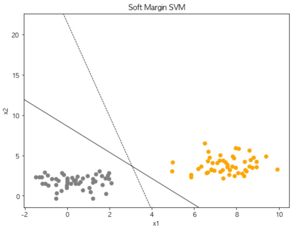
fig, ax = plt.subplots(figsize=(8,6))
ax.scatter('x1', 'x2', data=df[df['y']==1], color='orange')
ax.scatter('x1', 'x2', data=df[df['y']==-1], color='gray')

ax.set_xlabel('x1')
ax.set_ylabel('x2')
ax.set_title('Soft Margin SVM')

ax.axline((0, intercept1), slope=slope1, color='black', linewidth=0.8)
ax.axline((0, intercept2), slope=slope2, color='black', linestyle='dashed', linewidth=0.8)
plt.show()

Reference
Hastie, T., Tibshirani, R.,, Friedman, J. (2001). The Elements of Statistical Learning. New York, NY, USA: Springer New York Inc..
'Machine Learning' 카테고리의 다른 글
| Smoothing Splines & Smoother Matrices (0) | 2022.06.09 |
|---|---|
| Basis Expansions & Regularization (0) | 2022.06.09 |
| Linear Classifier (1) (0) | 2022.05.27 |
| Orthogonalization (0) | 2022.05.27 |
| Linear Method (0) | 2022.05.27 |


